第2部 R言語のデータ処理
wass80
2017-03-10
Rでデータ処理
生データから情報を取り出す
ライブラリを使う
これら全部がHadleyの作っているtidyverseライブラリ群
Hadley?
- Rの神
- データ解析用の様々なライブラリを提供している
R for Data Science
Hadleyの書いたこの本を元にやっていく
とりあえず実践
Rに組み込まれているデータを使う
- iris あやめのガク(Sepal)と花弁(Petal)と品種のデータ
- esoph タバコと酒とガンのデータ
などが組み込まれている
iris
##   Sepal.Length Sepal.Width Petal.Length Petal.Width Species
## 1          5.1         3.5          1.4         0.2  setosa
## 2          4.9         3.0          1.4         0.2  setosa
## 3          4.7         3.2          1.3         0.2  setosa
## 4          4.6         3.1          1.5         0.2  setosa
## 5          5.0         3.6          1.4         0.2  setosa
## 6          5.4         3.9          1.7         0.4  setosa

データフレーム
## 'data.frame':    150 obs. of  5 variables:
##  $ Sepal.Length: num  5.1 4.9 4.7 4.6 5 5.4 4.6 5 4.4 4.9 ...
##  $ Sepal.Width : num  3.5 3 3.2 3.1 3.6 3.9 3.4 3.4 2.9 3.1 ...
##  $ Petal.Length: num  1.4 1.4 1.3 1.5 1.4 1.7 1.4 1.5 1.4 1.5 ...
##  $ Petal.Width : num  0.2 0.2 0.2 0.2 0.2 0.4 0.3 0.2 0.2 0.1 ...
##  $ Species     : Factor w/ 3 levels "setosa","versicolor",..: 1 1 1 1 1 1 1 1 1 1 ...
- data.framecというclassのlist
- 要素のvectorはすべて同じ長さ
- Rでのデータの表現でよく使われる
とりあえずプロットしないことには
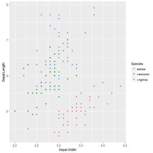
library(ggplot2)
ggplot(iris) +
  geom_point(aes(x = Sepal.Width, y = Sepal.Length,
                 color = Species))
キモい構文
ggplot(iris) +
  geom_point(aes(x = Sepal.Width, y = Sepal.Length,
                 color = Species))
- 演算子オーバーロードです
ggplot(data)でプロットするデータを指定+でレイヤーを重ねるpointが追加されているpointの属性にはx,y.color,size等がある
aes データ系列
- データに依存する値を指定する
- 共通の値は
aesに入れない
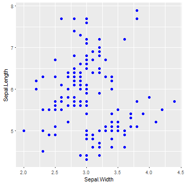
ggplot(iris) +
  geom_point(aes(x = Sepal.Width, y = Sepal.Length),
             color = "blue", size = 2)
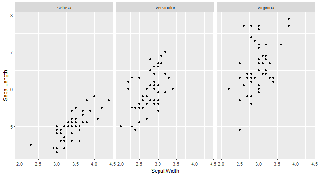
系統ごとにplot (facet)
ggplot(iris) +
  geom_point(aes(x = Sepal.Width, y = Sepal.Length)) +
  facet_wrap(~ Species)
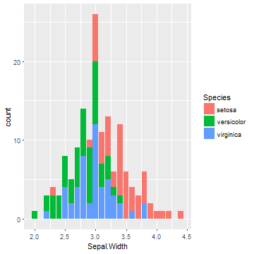
ヒストグラムも (stat)
- ヒストグラムのためには値を区切って数える前処理が必要になる
statで前処理を指定, x, yを求めてくれる- (
geom_barでは実はデフォルト)
ggplot(iris) +
  geom_bar(aes(x = Sepal.Width, fill = Species),
           stat = "count")
dplyrでデータ変形
library(nycflights13)
flights
## # A tibble: 336,776 × 19
##     year month   day dep_time sched_dep_time dep_delay arr_time
##    <int> <int> <int>    <int>          <int>     <dbl>    <int>
## 1   2013     1     1      517            515         2      830
## 2   2013     1     1      533            529         4      850
## 3   2013     1     1      542            540         2      923
## 4   2013     1     1      544            545        -1     1004
## 5   2013     1     1      554            600        -6      812
## 6   2013     1     1      554            558        -4      740
## 7   2013     1     1      555            600        -5      913
## 8   2013     1     1      557            600        -3      709
## 9   2013     1     1      557            600        -3      838
## 10  2013     1     1      558            600        -2      753
## # ... with 336,766 more rows, and 12 more variables: sched_arr_time <int>,
## #   arr_delay <dbl>, carrier <chr>, flight <int>, tailnum <chr>,
## #   origin <chr>, dest <chr>, air_time <dbl>, distance <dbl>, hour <dbl>,
## #   minute <dbl>, time_hour <dttm>
データテーブル
- R標準のデータフレームは遅いので, Hadleyの提供する
data.tableを使う
- データフレームより制約が柔軟で, 速く処理できる
- 特にファイル入出力が速い
## Classes 'tbl_df', 'tbl' and 'data.frame':    336776 obs. of  19 variables:
##  $ year          : int  2013 2013 2013 2013 2013 2013 2013 2013 2013 2013 ...
##  $ month         : int  1 1 1 1 1 1 1 1 1 1 ...
##  $ day           : int  1 1 1 1 1 1 1 1 1 1 ...
##  $ dep_time      : int  517 533 542 544 554 554 555 557 557 558 ...
##  $ sched_dep_time: int  515 529 540 545 600 558 600 600 600 600 ...
##  $ dep_delay     : num  2 4 2 -1 -6 -4 -5 -3 -3 -2 ...
##  $ arr_time      : int  830 850 923 1004 812 740 913 709 838 753 ...
##  $ sched_arr_time: int  819 830 850 1022 837 728 854 723 846 745 ...
##  $ arr_delay     : num  11 20 33 -18 -25 12 19 -14 -8 8 ...
##  $ carrier       : chr  "UA" "UA" "AA" "B6" ...
##  $ flight        : int  1545 1714 1141 725 461 1696 507 5708 79 301 ...
##  $ tailnum       : chr  "N14228" "N24211" "N619AA" "N804JB" ...
##  $ origin        : chr  "EWR" "LGA" "JFK" "JFK" ...
##  $ dest          : chr  "IAH" "IAH" "MIA" "BQN" ...
##  $ air_time      : num  227 227 160 183 116 150 158 53 140 138 ...
##  $ distance      : num  1400 1416 1089 1576 762 ...
##  $ hour          : num  5 5 5 5 6 5 6 6 6 6 ...
##  $ minute        : num  15 29 40 45 0 58 0 0 0 0 ...
##  $ time_hour     : POSIXct, format: "2013-01-01 05:00:00" "2013-01-01 05:00:00" ...
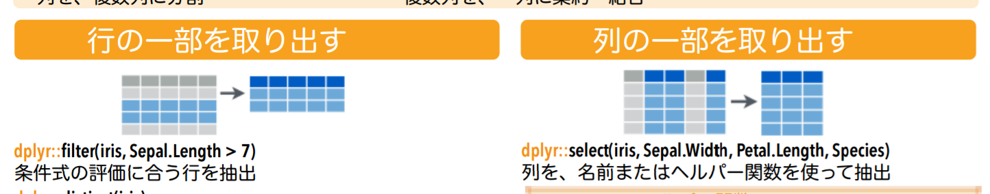
filter (行の抽出)
filter(flights, air_time < 100) #100分未満のフライト
## # A tibble: 105,687 × 19
##     year month   day dep_time sched_dep_time dep_delay arr_time
##    <int> <int> <int>    <int>          <int>     <dbl>    <int>
## 1   2013     1     1      557            600        -3      709
## 2   2013     1     1      559            559         0      702
## 3   2013     1     1      629            630        -1      721
## 4   2013     1     1      629            630        -1      824
## 5   2013     1     1      632            608        24      740
## 6   2013     1     1      639            640        -1      739
## 7   2013     1     1      643            645        -2      837
## 8   2013     1     1      645            647        -2      815
## 9   2013     1     1      732            735        -3      857
## 10  2013     1     1      733            736        -3      854
## # ... with 105,677 more rows, and 12 more variables: sched_arr_time <int>,
## #   arr_delay <dbl>, carrier <chr>, flight <int>, tailnum <chr>,
## #   origin <chr>, dest <chr>, air_time <dbl>, distance <dbl>, hour <dbl>,
## #   minute <dbl>, time_hour <dttm>
select (列の抽出)
select(flights, dep_time, arr_time) # 離発着時刻
## # A tibble: 336,776 × 2
##    dep_time arr_time
##       <int>    <int>
## 1       517      830
## 2       533      850
## 3       542      923
## 4       544     1004
## 5       554      812
## 6       554      740
## 7       555      913
## 8       557      709
## 9       557      838
## 10      558      753
## # ... with 336,766 more rows
つまり
arrange (並び替え)
arrange(flights, desc(arr_delay)) # 遅れた順
## # A tibble: 336,776 × 19
##     year month   day dep_time sched_dep_time dep_delay arr_time
##    <int> <int> <int>    <int>          <int>     <dbl>    <int>
## 1   2013     1     9      641            900      1301     1242
## 2   2013     6    15     1432           1935      1137     1607
## 3   2013     1    10     1121           1635      1126     1239
## 4   2013     9    20     1139           1845      1014     1457
## 5   2013     7    22      845           1600      1005     1044
## 6   2013     4    10     1100           1900       960     1342
## 7   2013     3    17     2321            810       911      135
## 8   2013     7    22     2257            759       898      121
## 9   2013    12     5      756           1700       896     1058
## 10  2013     5     3     1133           2055       878     1250
## # ... with 336,766 more rows, and 12 more variables: sched_arr_time <int>,
## #   arr_delay <dbl>, carrier <chr>, flight <int>, tailnum <chr>,
## #   origin <chr>, dest <chr>, air_time <dbl>, distance <dbl>, hour <dbl>,
## #   minute <dbl>, time_hour <dttm>
mutate (新しい列)
f <- select(flights, distance, air_time) # 距離と時間
mutate(f, speed = distance / air_time) # 速さ
## # A tibble: 336,776 × 3
##    distance air_time    speed
##       <dbl>    <dbl>    <dbl>
## 1      1400      227 6.167401
## 2      1416      227 6.237885
## 3      1089      160 6.806250
## 4      1576      183 8.612022
## 5       762      116 6.568966
## 6       719      150 4.793333
## 7      1065      158 6.740506
## 8       229       53 4.320755
## 9       944      140 6.742857
## 10      733      138 5.311594
## # ... with 336,766 more rows

%>%
- 他の言語で言うパイプ
- 右辺の返り値を左辺の第1引数にする
- tidyverseライブラリで提供されている
- 途中の一時変数がなくなる
## [1] 3
さっきと同じもの
flights %>%
  select(distance, air_time) %>% # select(flight, ...)
  mutate(speed = distance / air_time)
summarize (縮約)
flights %>%
  summarise(delay = mean(arr_delay, na.rm=TRUE)) # 平均遅れ
## # A tibble: 1 × 1
##      delay
##      <dbl>
## 1 6.895377

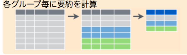
group_by
flights %>%
  group_by(dest) %>% # 目的地ごとに
  summarise(delay = mean(arr_delay, na.rm=TRUE)) # 平均遅れ
## # A tibble: 105 × 2
##     dest     delay
##    <chr>     <dbl>
## 1    ABQ  4.381890
## 2    ACK  4.852273
## 3    ALB 14.397129
## 4    ANC -2.500000
## 5    ATL 11.300113
## 6    AUS  6.019909
## 7    AVL  8.003831
## 8    BDL  7.048544
## 9    BGR  8.027933
## 10   BHM 16.877323
## # ... with 95 more rows
これSQLでは?
- 実際, sqlliteの操作などにも使える
- dplyrはデータベースに対する, 一般的なAPI
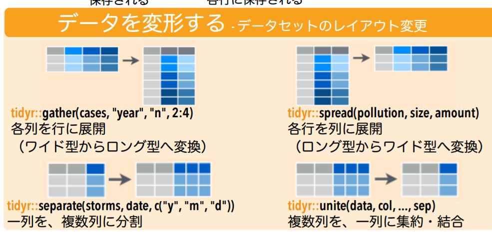
紹介: tidyr
- データの整形をして, dplyrで扱えるようにするライブラリ
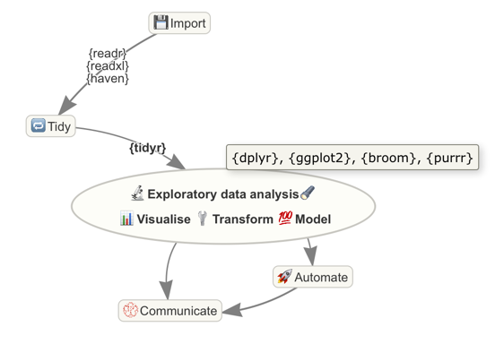
データ解析の流れ
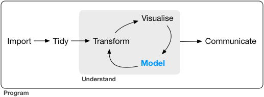
- ビジュアライズとデータ変形を見てきた
- ここからModelを見出すことでデータ処理が完了する
- Modelとは変数の関係性のこと
Modelの発見
- まず, モデル群を考える
Y = a_1 X + a_2Z = a_1 X * a_2 Y + a_3- など
- 次にデータに合う係数を見つける
実践
library(modelr)
ggplot(sim1) + geom_point(aes(x=x, y=y))
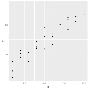
このデータに適合するモデルを考える
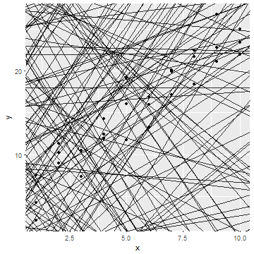
線形モデル
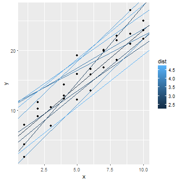
Y = a_1 X + a_2をモデル群として考える- ランダムに作った
model_aを係数として, どの直線が最も適合するか
model_a <- data.frame(a1 = runif(200, -5, 5),
                      a2 = runif(200, -20, 40))
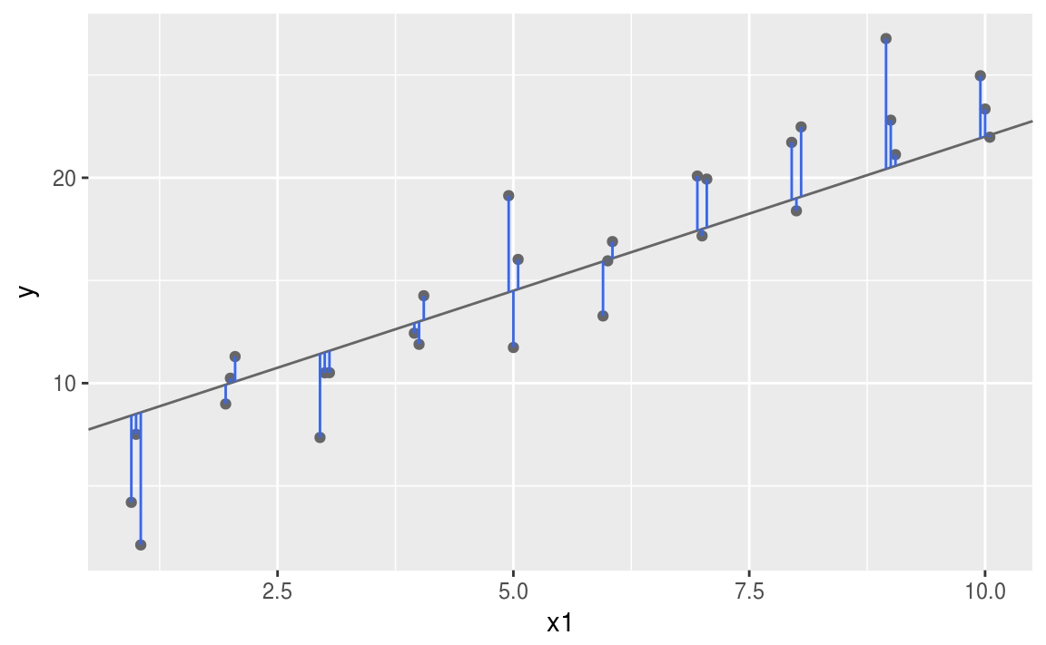
最小二乗法
- モデルに対して, Y軸での差の2乗の平均の平方根が小さいものが良いモデルとする
簡単にできるところまで
モデルを関数で定義
my_model <- function(a1, a2, data) a1 * data$x + a2
mini_data <- data.frame(x=c(1,2), y=c(3,5))
my_model(2, 5, mini_data)
## [1] 7 9
Y軸での差を求める
measure_distance <- function(a1, a2) {
  diff <- sim1$y - my_model(a1, a2, sim1)
  sqrt(mean(diff ^ 2)) # 各要素の2乗の平均の平方根
}
差を求めてみる
model_a <- model_a %>%
  mutate(dist = purrr::map2_dbl(a1, a2, measure_distance))
- distで先程のmodelの直線をを色付
- 黒いものほど, 適合したmodelと言える
実際に求める
lmにモデル群とデータを渡す
sim1_a <- lm(y ~ x, data = sim1)
sim1_a$coefficients
## (Intercept)           x
##    4.220822    2.051533
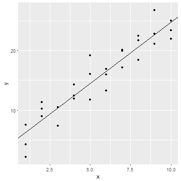
良さそう
まとめ: モデル
- データから結論を見つける
- モデルは線形以外にも多く有る
大まとめ
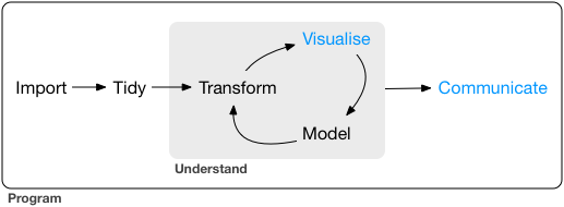
- データ解析の流れとして以下を見てきた
- 整形: tidyr
- ビジュアライズ: ggplot
- 変形: dplyr (+ purrr)
- モデル: Modelr (+ broom)
- Haddlyさんは情報発信まで含めてデータ解析と言ってる
ところで
- さっきから出てくる構文気持ち悪く無いですか?
y ~ xって何?aes(x = x, y = y), data = sim1も不思議library(dplyr)も変では%>% ってどうやって定義されてるの
- メタプログラミング編へ